P4 — Global Navigation
Gradient Navigation with Cost Expansion Using BFS
This blog describes how to implement a gradient navigation system for a mobile robot, combining two approaches: cost expansion with BFS and gradient navigation. The system enables the robot to move efficiently towards a target, avoiding obstacles, while continuously following the path of least cost dynamically calculated.
Introduction
Instead of planning an entire path before starting, this approach combines BFS-based cost expansion to calculate the map’s cost from the target to the robot, and then uses gradient navigation to move continuously following the cost map. The gradient guides the robot toward the target while avoiding obstacles, and the BFS algorithm ensures that the costs on the map are consistent and correctly reflect the proximity to the target.
System Features:
- Cost Expansion with BFS: BFS is used to calculate the cost of each cell on the map from the target to the robot, ensuring that the path to the target always has the least cost.
- Obstacle Inflation: The cost of cells near obstacles is increased to prevent the robot from getting too close to them.
- Gradient Navigation: Once the cost map is computed, the robot uses the gradient of the map to move towards the target, following the path of least cost.
- Dynamic Updates: The system allows the target to be updated in real time, adapting to changes in the environment.
Process Description
1. Loading the Map
The environment map, loaded from a grayscale image, represents free areas (value 255) and obstacles (value 0). This map is converted into a cost grid, where the cost of each cell is determined by its distance from the obstacles.
2. Cost Expansion with BFS
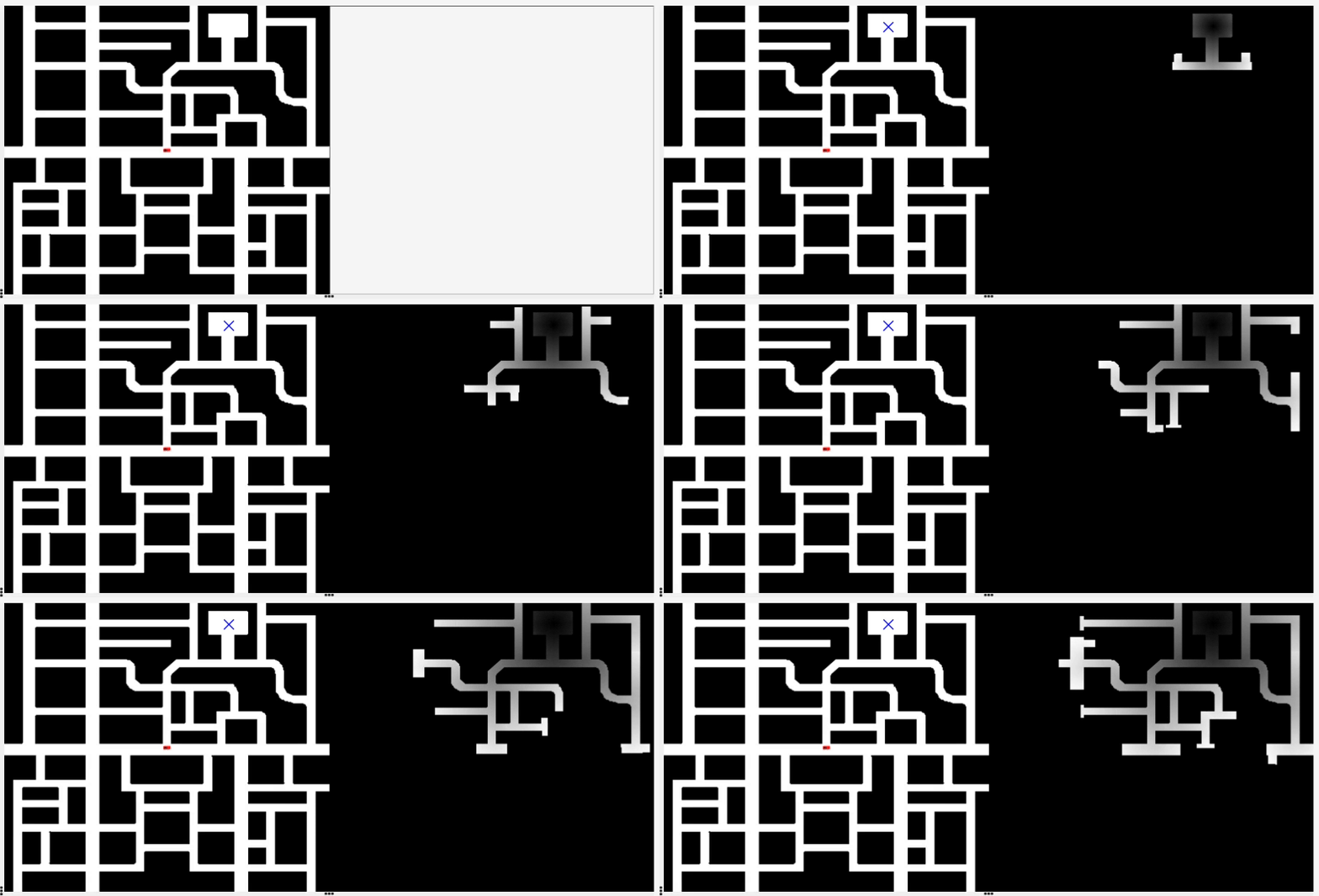
To calculate the cost map, BFS is used, starting from the target and expanding backwards to the robot. The idea is to assign a cost to each cell that indicates the minimum distance to the target, with the cost being 0 for the destination cell.
3. Obstacle Inflation
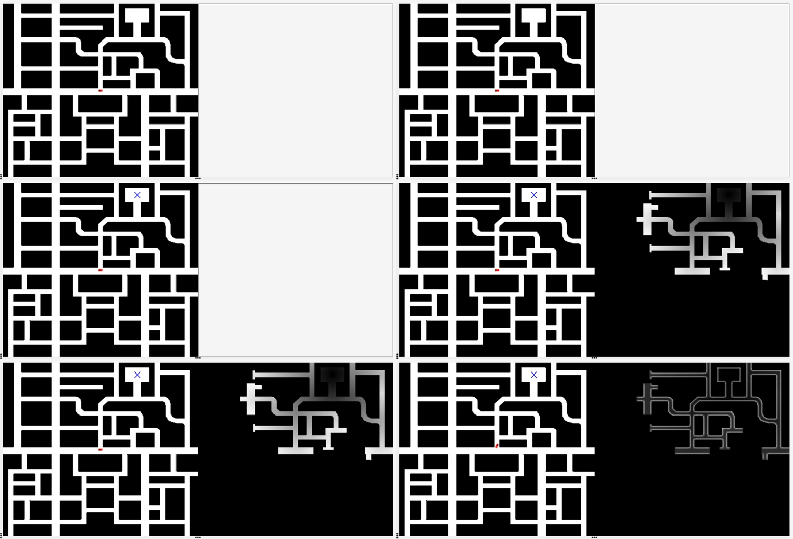
Obstacle inflation is applied to ensure that the robot does not get too close to obstacles. This process increases the cost of cells near obstacles, creating a “safety zone” around them. The MAX_INFLATION parameter controls the size of this zone.
Expansion Process:
- Start at the target cell, assigning a cost of 0.
- BFS then expands to neighboring cells, incrementing the cost of each cell based on its distance from the target.
- The process continues until all relevant cells have an assigned cost, creating a cost map that reflects the “cheapest path” to the target.
This step is crucial because it ensures that the robot has an accurate and optimized cost map to guide its movement.
4. Gradient Navigation
Once the cost map is generated, the robot uses gradient navigation to move towards the target. The gradient is calculated in real time from the cost values of neighboring cells.
Gradient Calculation:
- The robot evaluates neighboring cells in the 8 possible directions (cardinal and diagonal).
- It moves towards the cell with the lowest cost (the least gradient).
- This process is repeated continuously, adjusting the direction based on the costs of nearby cells.
5. Dynamic Target Update
The system allows the target to change during navigation. If the robot’s target changes, the BFS expansion process is repeated to recalculate the costs and the gradient, ensuring that the robot always follows the most efficient path according to the new information.
6. Robot Movement
The robot uses the calculated gradient to adjust its speed and direction, moving towards the cell with the least cost at each step. This ensures that the robot moves efficiently, avoiding obstacles, and adjusting its heading based on the environment’s conditions.
Process Summary
- Load the map: An image representing the environment is loaded and converted into a cost map.
- Cost expansion with BFS: The BFS algorithm expands the cost map from the target to the robot, ensuring that the path to the target is the least expensive.
- Obstacle inflation: The costs of cells near obstacles are increased to ensure the robot avoids getting too close.
- Gradient navigation: Using the cost map generated by BFS, the robot navigates towards the target by following the gradient of the least cost.
- Dynamic updates: If the target changes, the costs and the gradient are recalculated, allowing the robot to adapt to the new environment.
- Robot movement: The robot adjusts its speed and direction based on the gradient, ensuring it follows the least-cost path while avoiding obstacles.
Videos
- Test linear_vel = 5:
- Test linear_vel = 4:
Conclusion
The system described in this blog combines two navigation techniques: cost expansion with BFS and gradient navigation. First, BFS is used to calculate the costs from the target to the robot, ensuring that the robot moves along the least-cost path. Then, the robot uses the gradient of this map to navigate efficiently, avoiding obstacles and adjusting its trajectory in real time. This approach is flexible and efficient, allowing the robot to adapt to changes in the environment while moving towards its target.